In this post, I want to give a clear explanation of what artificial neural networks are, how they work, and present a few different perspectives on why they work, from linear algebra to logic circuits. You do not need to have any real previous knowledge, just some basic maths understanding.
Introduction
Artificial neural networks (ANNs) have been around for a long time (since the middle of last century!), but have gained in popularity at the end of the 80s, and once again more recently with the introduction of deep learning.
As the name suggests, ANNs are artificial representations of biological neural networks, an intricate network of interconnected neurons that constitutes the nervous system of human beings and animals.
The basic ability of a neural network is that of making an “inference” about something that gets fed to it.
A very common example is a network that distinguish between pictures of cats and dogs (because everyone on the internet loves pets, right?):
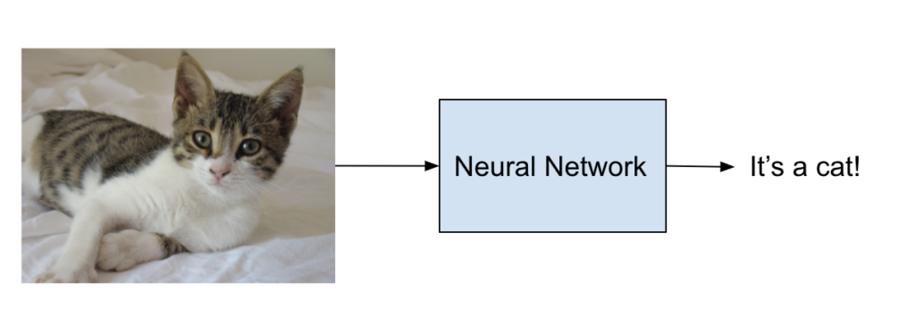
The network is inferring if the picture is one of a cat or a dog.
An interesting behaviour of a neural network is that we can train it on some examples so that it can adapt to solve different problems. If, for example, we feed many images of cats and dogs and tell the network what they are, it will start distinguish them. If we train a network with the same structure on different categories, let’s say cars vs airplanes, the network will learn how to distinguish between those two categories.
The input of a network can be anything representable by numbers. In our examples each image is encoded by a sequence of numbers. The network will then process those numbers and find a mathematical way to distinguish the examples we have.
There is another nice effect that neural networks usually achieve to a certain degree: generalisation. That means that if I show the network enough images of cats and dogs it will probably make the right decision on a new image even if it’s never seen that particular image before. However, this is not guaranteed.
The building blocks: neurons
Let’s start with the simplest unit, the building block of a neural network: a neuron.
The following picture shows a model of a neuron:
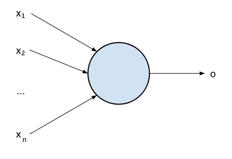
Its function is very simple: it takes some inputs x_i and it produces an output o according to the value of the inputs.
First mathematical notation
Let’s try to use a mathematical notation to represent that. What is it in maths that takes some inputs and produces an output? A function!
So we can easily represent a neuron as a function f of some inputs x_1, …, x_n:
f(x_1, x_2, …, x_n)Using mathematical notation will help us later on to understand some nice properties of the neuron, but remember: it’s just a way of representing that within a system that we know well, nothing more.
Let’s now have a look at what happens inside: our neuron will sum up all its inputs to produce the output. This is not just a sum though but a weighted sum: before summing, every input is weighted. This is because an input might be more important than another for that neuron.
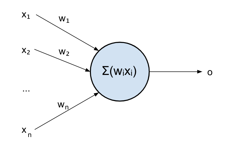
Mathematically, this can be expressed as follow:
f(x_1, x_2, …, x_n) = w_1 x_1 + w_2 x_2 + … + w_n x_nOr with a more compact notation:
f(x_1, x_2, …, x_n) = \displaystyle\sum_{i}w_i x_iWhere w_i are the weights for each input x_i
OK, so a neuron simply combines its inputs in a weighted manner to produce an output. But why is that useful? What can be achieved with it?
Well, not much yet, it’s just doing what in maths is called a “linear combination“.
The AND example
Let’s see a practical example. Let’s assume I want to cross a two-way road. I’ll need to look at both sides, and only when I can see that no car is coming from any of the sides I will start crossing.
Logically, we can write this as follows:
If condition1 is true AND condition2 is true then cross the road
Where each condition is that no car is coming from that side of the road.
This is what it’s called a logical AND.
Let’s represent true by 1 and false by 0.
To cross the road, I need a function that gives me 1 if the two inputs are 1, and 0 otherwise.
Let’s write what it’s called a “truth table” for our AND gate to understand what the outputs should be for each combination of inputs:
| x1 | x2 | AND(x1, x2) |
| 0 | 0 | 0 |
| 1 | 0 | 0 |
| 0 | 1 | 0 |
| 1 | 1 | 1 |
This is a bit like the cats vs dogs example I mentioned earlier: I’m trying to use the neuron to distinguish between one kind of inputs (1, 1) vs the others.
Unfortunately, my neuron cannot do that just yet: even if we set the weights to 0.5, the result of the combination will be the following:
| x1 | x2 | f(x_1, x_2) = 0.5x_1 + 0.5x_2 |
| 0 | 0 | 0 |
| 1 | 0 | 0.5 |
| 0 | 1 | 0.5 |
| 1 | 1 | 1 |
Close enough, but we wouldn’t know what to do in case a car is coming from only one side of the road.
Sure, I could set each w to something like 0.3, so to have 0.3 (which is closer to 0) in case only one input is active, and 0.6 (which is closer to 1) if both inputs are active. This way, if I can round off the output to the closest integer the neuron would produce the expected result.
The real problem is that no one is there for us to do that rounding. We will need to include an additional piece to our neuron that can do that.
If you think about it, that’s where the real decision comes in, we need something that compares the output of our linear combination, and decides if it’s greater than 0.5 and only in that case fire out a response from the neuron.
That part is called the activation function.
The activation function
As the word suggests, the activation function “activates” when its input reaches a certain value.
There are many functions that can work well for that, but one of the first to be used in neural networks was the sigmoid function. That choice was done for a few different reasons: because it’s differentiable (this will be useful later on), its output is bounded between 0 and 1 (very good for representing logic circuits) and also for its resemblance to how the neural cells actually work.
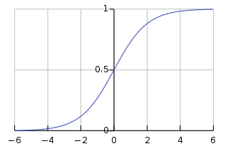
The sigmoid function takes an input in ]-inf, +inf[ and maps it to ]0, 1[
So the function of our neuron will now look like:
f(x_1, x_2) = sigmoid(w_1 x_1 + w_2 x_2)
Out updated model of a neuron will look like this:
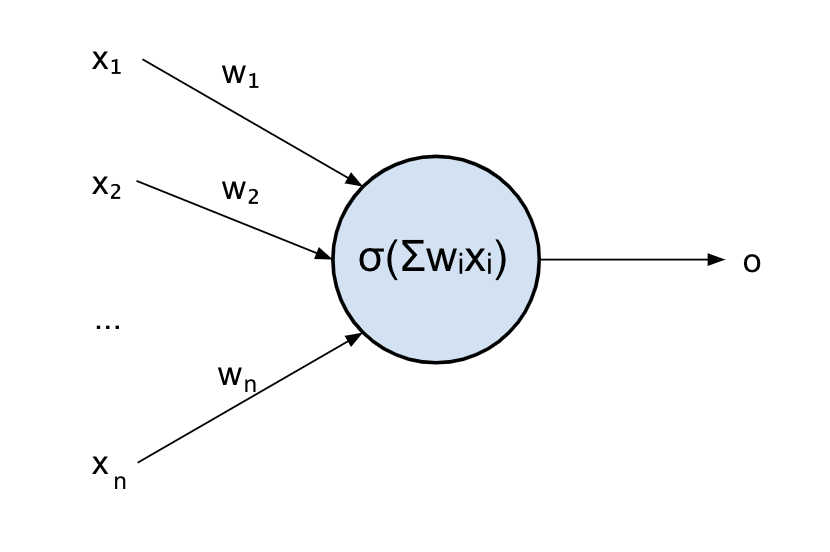
Where \displaystyle\sigma is the activation function of the neuron.
The problem of the sigmoid is that it is not very steep around 0, this means we would need to increase our weights for the example to work well, or use a steeper activation function.
Also, the sigmoid is centred around 0, so that sigmoid(0) = 0.5. This will not work for our example, since we want f(0.5) as close to 0 as possible.
The bias
Let’s introduce the last missing piece, the “bias”.
You can imagine a bias being an input that is always set to a certain value and adds that value to the combination that the neuron computes:
f(x_1, x_2) = sigmoid(w_1 x_1 + w_2 x_2 + b)
Where b is our bias.
Our final model of the neuron will look like this:
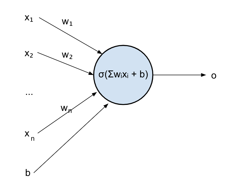
In maths, the input of the sigmoid w_1x_1 + w_2x_2 + b is still just a linear combination.
We can now set our weights to something high like 10, just so we can saturate our sigmoid and have its output as close to 1 or 0 as possible and shift the sigmoid input back by 15 to have something closer to the boundaries:
| x1 | x2 | f(x_1, x_2) = sigmoid(10x_1 +10x_2 – 15) |
| 0 | 0 | 0.00.. |
| 1 | 0 | 0.00.. |
| 0 | 1 | 0.00.. |
| 1 | 1 | 0.99.. |
That worked! We managed to reproduce the AND table with an artificial neuron.
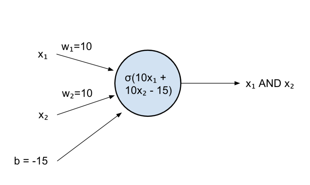
We had to mess around with the weights and bias a bit, but this is where things get interesting: a neural network, like the brain, should be able to learn from examples.
This means that you should be able to start from any random weights and bias, feed lots of examples of an AND (well, there are only 4 possible examples in this case but you get the point), and after a while the network will learn by itself the best possible weights and bias to produce the expected output.
Training a neural network is something I will not go into details in this post for now.
But let’s get back to our example: why was it so important that our single neuron could learn to perform an AND operation?
Well, logic gates (AND, OR, XOR, etc) are the basis of computers. If you combine many of those together, you can perform complex logical operations.
If we start connecting neurons together, we will expect our network of neurons to be able to learn more complex operations, hence becoming smarter and smarter!
Another perspective: linear separability
For simplicity, instead of sigmoid, I will use a Heaviside step function as our activation function.
This is a much easier function to reason with (but not really used in practice for many problems, like non differentiability and leading to vanishing gradients – don’t worry about that for now!).
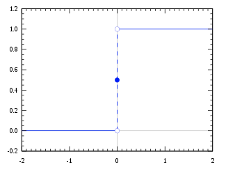
It’s a very simple function that outputs 1 if the input is >=0 and 0 otherwise.
That means our AND neuron could just be:
f(x_1, x_2) = heaviside(x_1 + x_2 – 1.5)
Let’s now plot all possible values of x_1 and x_2 on a cartesian plane:
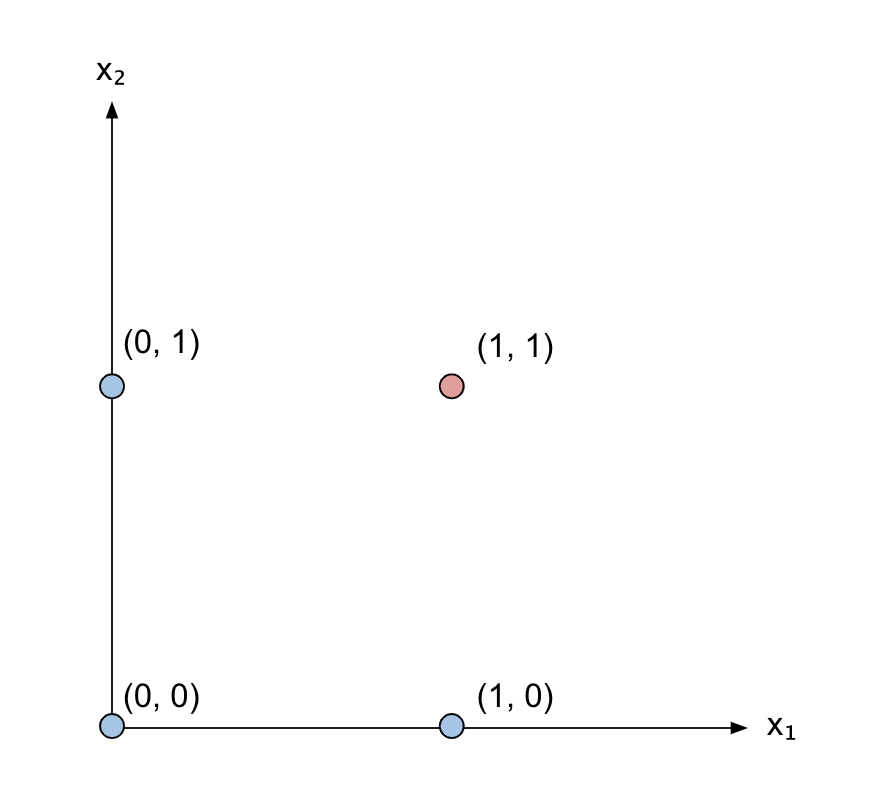
I’ve coloured in red the point (1, 1) that activates the AND gate, giving an output of 1, and in blue all the other points that give an output of 0.
Remember the equation of a line: y = ax + b where a determines the slope and b how much shift from the origin the line has.
Now, let’s think about the linear combination happening in our AND neuron as a line:
x_1 + x_2 – 1.5 can actually be written as x_2 = -x_1 + 1.5, so that it’s clear it represents a line with negative slope and shifted by 1.5:
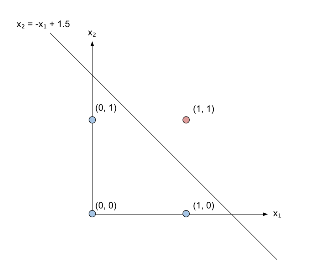
Can you see what’s happening there? Our linear combination of the inputs corresponds to the line that separates the point we are interested in (1, 1) which is the only one that satisfies the AND relation from the other three points.
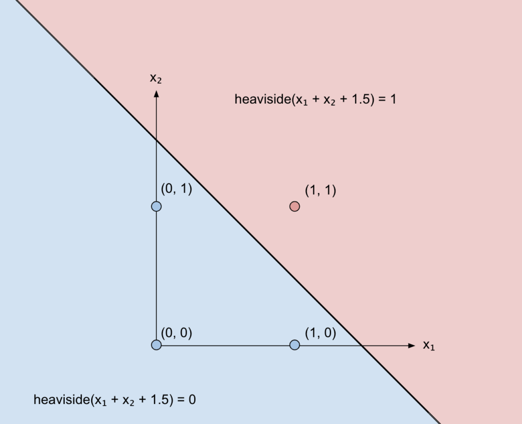
Applying the Heaviside function means that everything above that line will be 1, and everything below will be 0.
You would need three axes to visualize that, since two axes are x1 and x2 and the third is the output value of the heaviside function. But since that value is either 0 or 1, we can just use two different colours and keep our nice 2-D plane to visualize what’s happening:
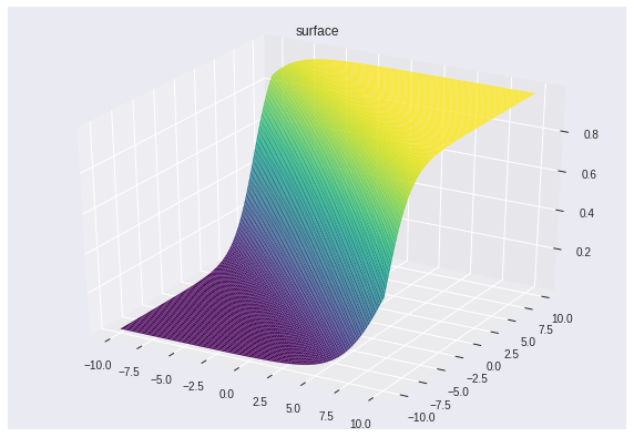
That’s also why I didn’t use the sigmoid function. It would have been difficult to visualize in 2-D. Instead, you would have seen a 3-D version of the sigmoid, something like this:
Classification vs Regression
So, the line parametrized by weights and bias acts as a separator between the “good’ points (the ones we want to assign 1, so to make them pass) and the “bad” points.
This kind of problem, where you want to separate some points into two “classes”, is also called a binary classification problem: classification since we want the points to belong to a “class”, binary since we only have good vs bad points (0 vs 1), so two classes.
Of course, we can have classification problems with multiple classes. We can also have problems that are not classification, where instead of assigning a point to a class we assign it to a real number. These problems are called regression problems. Applying a sigmoid instead of the heaviside, for example, would have done that (remember that the outputs of the sigmoid are real values in ]0, 1[).
An example of a classification problem can be distinguishing between images of cats vs dogs. You only have two classes, the “cat” class and the “dog” class. Of course, you’ll end up representing cats and dogs by a number, like our 0 and 1.
An example of a regression problem is guessing the height of a person from a picture.
So, to recap, the weights and the bias act on that separation line as you would expect from the equation of a line: weights determine the inclination and the bias the shift.
So, training a neuron can also be seen as constantly rotating and shifting that line until you find a line that can separate well the examples you have.
Obviously, there’s more than one solution in our case.
The problem of noisy data
In real-life examples, there’s also another problem: the data you have is noisy. In our AND problem, we only could feed 4 examples to the neuron, the 4 pairs of binary inputs. But imagine if you couldn’t really be sure if a car was coming or not. You would have some real numbers instead of 0s and 1s to model the uncertainty.
Even worse, in real life some data points might even be wrong, so you want to find a line that separates the majority of the points, but maybe it’s fine if some of those points are left in the wrong region.
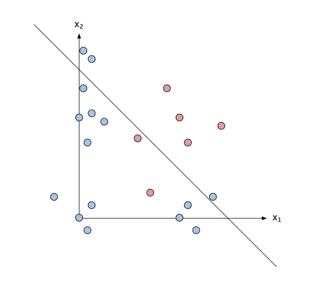
So far, we’ve only talked about one neuron. You can easily combine more neurons to get something more complex.
A bit about generalisation
Let’s consider the figure above, but this time let’s imagine those examples are not just observations of logic values but some representation of cats and dogs. For example, x_1 could be the hight of the animal in the picture, and x_2 could be the size of the ears.
We might have found a line that can separate most of our training examples, finding that most dogs are bigger and have bigger ears, although not all of them.
After training, when the w and b of the line have been fixed, we present new examples and see how good that line is to separate these new examples: most likely, it will be quite good, since even the dogs we haven’t used for training are likely to be bigger and have bigger ears. This is what we mean by generalisation: finding a function that performs well even on samples we have not seen before.
I will talk more about generalisation in the next post, when I’ll go in-depth into how to train a network and present concepts like overfitting, validation, and more.
The XOR example – a complete Neural Network
Let’s try a more difficult example, the XOR gate.
The truth table for XOR looks like the following:
| x1 | x2 | XOR(x1, x2) |
| 0 | 0 | 0 |
| 1 | 0 | 1 |
| 0 | 1 | 1 |
| 1 | 1 | 0 |
Basically, it will output 1 if only one of the two inputs is true. But if they are both true, it will output 0.
A XOR can be reduced using OR, AND and NOT like the following:
x1 XOR x2 = (x1 OR x2) AND NOT(x1 AND x2)
We already know how an AND neuron looks like:
and(x_1, x_2) = h(x_1 + x_2 – 1.5)
Where h denotes the Heaviside function.
The OR neuron can be expressed like this (you can write down the truth table if you don’t believe me):
or(x_1, x_2) = h(x_1 + x_2 – 0.5)
We do need to invert the first AND in order to include the NOT (forming what it’s called a NAND gate), but we can do this by setting the weights to -1 and the bias to 1.5:
nand(x_1, x_2) = h(-x_1 – x_2 + 1.5)
Composing the above functions together, we obtain:
xor(x_1, x_2) = h(h(x_1+x_2-0.5)+h(-x_1-x_2+1.5)-1.5)
We can now create our XOR neural network by connecting all the neurons together like the following:
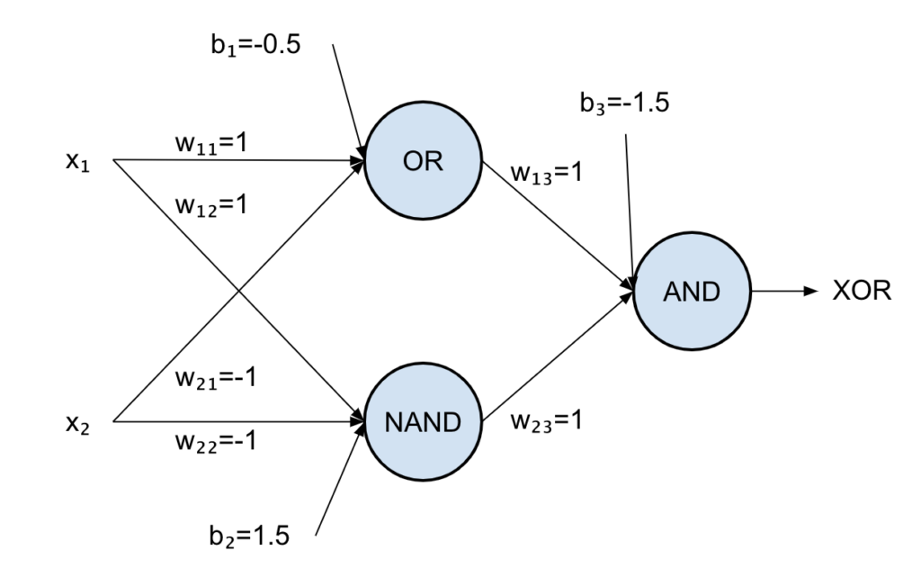
The first neuron is the OR gate, the second is the NAND and the last is an AND.
If you write the truth table of the above you will see that it corresponds to the XOR one!
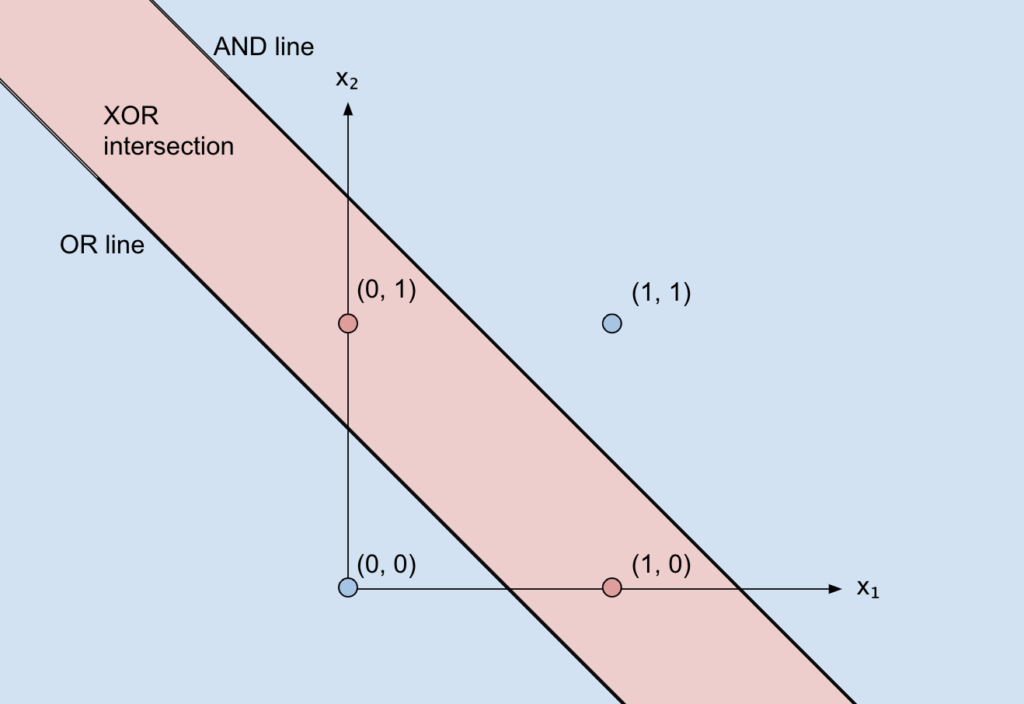
But let’s move onto the cartesian plane:
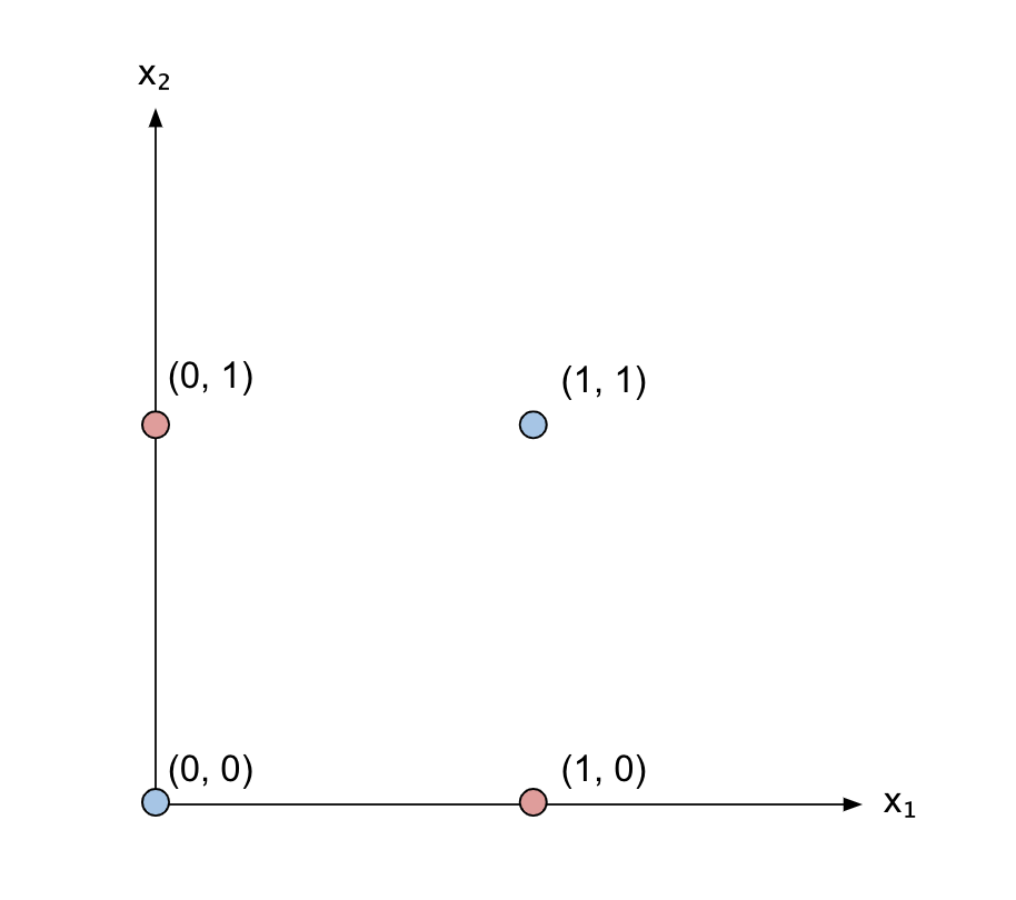
We’ll now need our function (the output of the network) to be 1 only for the points (1, 0) and (0, 1).
Hence, we need a way to separate those two points from the remaining two.
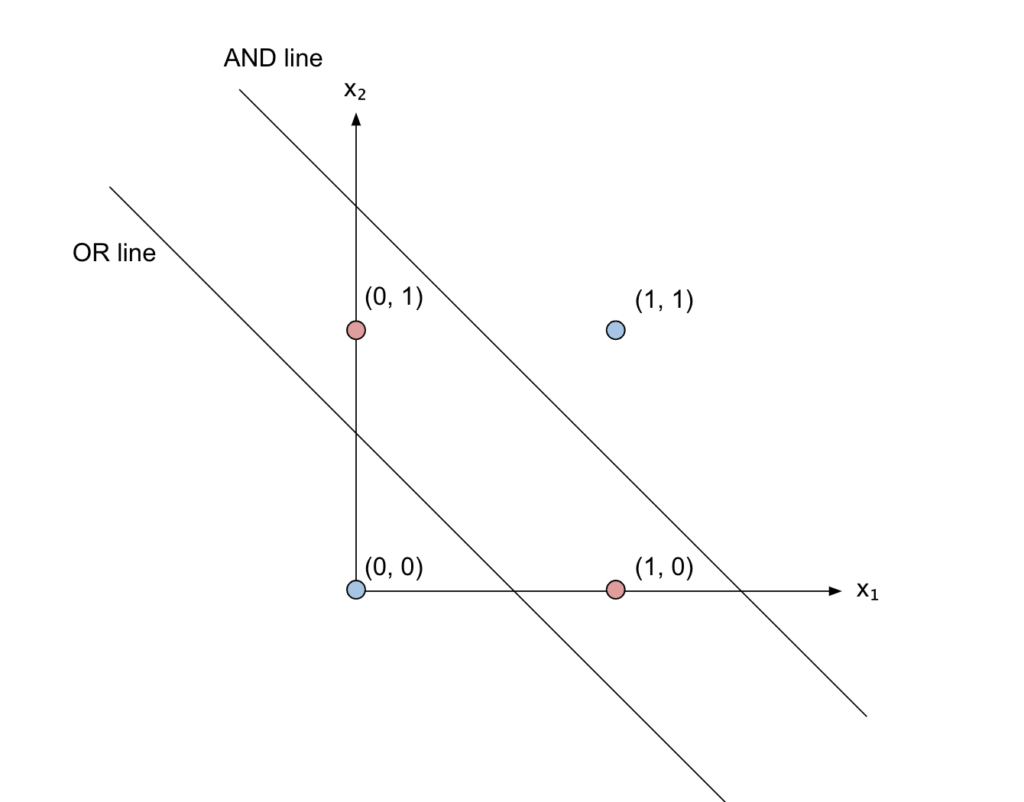
But, wait a second… that’s impossible with just one line!
We need two lines, which in our network corresponds to the OR neuron and the NAND neuron, and then we need to only consider the overlap of the part above the OR line and below the AND line (since it’s below and not above we have used a NOT). That overlap is achieved with the final AND.
Let’s have another look at the structure of our network:
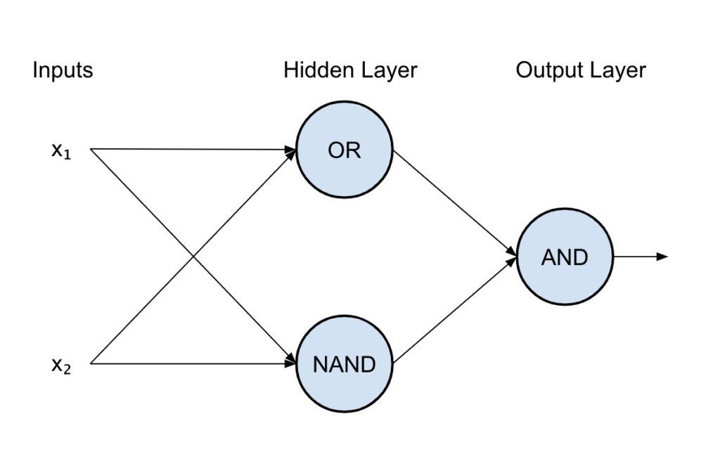
There are different nomenclatures and ways of counting layers, but we can say that this network has 2 layers: the first layer (with the OR and NAND neurons), also called the “hidden” layer since it’s hidden between the inputs and the outputs, and an output layer (AND).
This way, you can create any logic circuit you want, simulating any logic expression!
Was it possible to do that with just one layer? Well, not really. Otherwise, how could you combine the outputs together?
But how many layers do you need? Theoretically, only two! This result corresponds to the universal approximation theorem, which I won’t demonstrate here, but it’s very easy to see for logic circuits:
Any logic expression can be written as a combination of OR, NOT and AND. If you think about it, you’ll always have one layer that can compute all the ANDs and one that will compute all the ORs, e.g.:
x_1x_2x_3 + -x_2x_4 + x_5x_6
It is, however, easier to train “deeper” networks (made by more layers), since they can more easily capture complex structures (each layer will spot patterns in patters of patterns etc).
I will leave the intuition hanging for now, but I’ll come back to it later.
Neural networks and linear transformations
If you’re not familiar with vectors and linear algebra feel free to skip this section.
Let’s consider the first layer of our two-layer network that solves the XOR problem: we have our set of inputs, x_1 and x_2, and two weights for each neuron, w_11 and w_12 for the first neuron and w_21 and w_22 for the second.
Each neuron produces an output, o_1 and o_2, that will be then fed into the final layer.
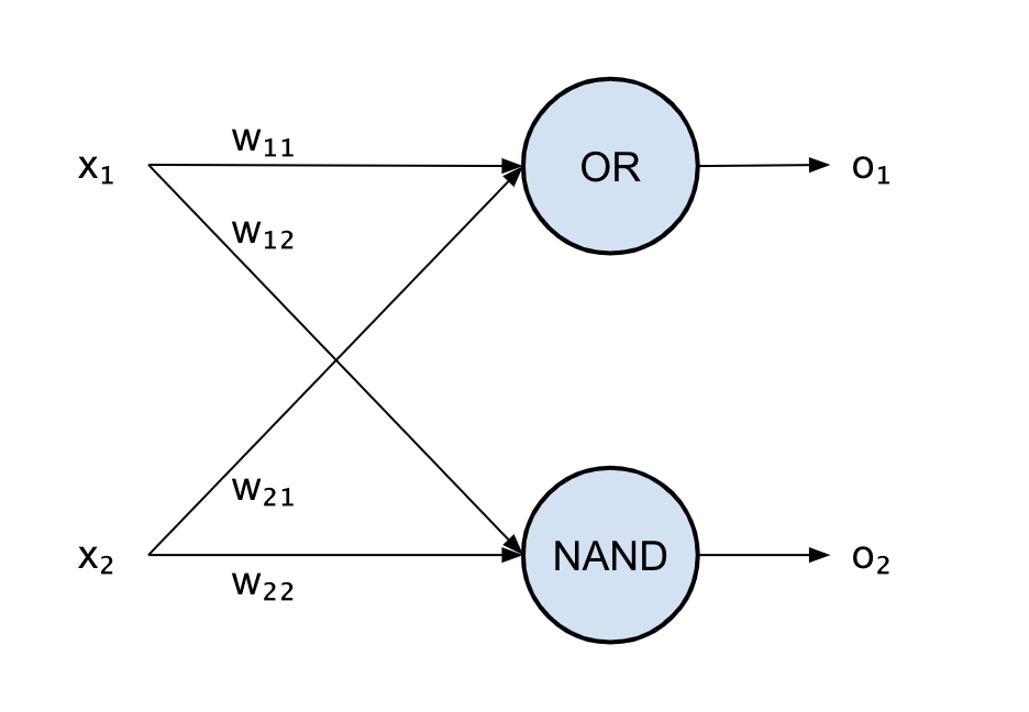
Remember: each neuron performs a linear combination and then applies a non-linear activation function.
Each linear combination can also be written as dot product in the Euclidean space between the input vector \vec{x} and weight vector \vec{w}, so that the output of the first neuron becomes:
o1 = h(\vec{x} \cdot \vec{w}) = h(w_1 x_1 + w_2 x_2) = h([x_1, x_2] \begin{bmatrix}w_{11} \\ w_{12}\\ \end{bmatrix})
The nice thing about this notation is that we can write the whole first layer as a matrix multiplication just by concatenating the two weight vectors corresponding to the two neurons in the first layer, obtaining a weight matrix for the first layer: W = \begin{bmatrix}w_{11} & w_{21} \\ w_{12} & w_{22}\\ \end{bmatrix}
Hence, the output of the first layer [o_1 o_2] becomes:
[o_1 o_2] = h(\vec{x} W) = h([x_1 x_2] \begin{bmatrix}w_{11} & w_{21} \\ w_{12} & w_{22}\\ \end{bmatrix})
The next figure shows the matrix multiplication between the input and the weight matrix, explaining the different dimensions:
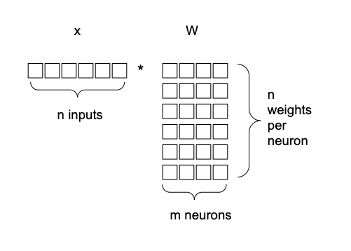
But \vec{x} W is nothing else than applying a linear transformation defined by W to the input vector \vec{x}.
A linear transformation just rotates and scales the input vector. Let’s not forget that we also add a bias, but that simply makes the transformation affine.
If there weren’t non-linearities in our network, every layer would just perform an affine transformation, so the whole network would be a composition of many affine transformations. But the composition of affine transformations can also be reduced to only one affine transformation!
This means that, without non-linearities, a network of one layer could do everything a network of any number of layers would do.
Thanks to non-linearities, we have more power than a simple affine transformation of the inputs.
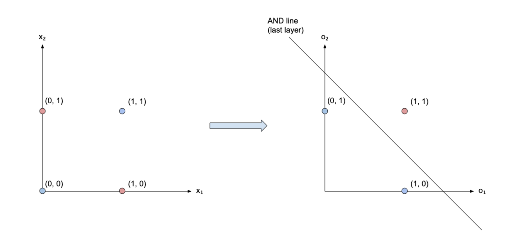
Intuition: the whole idea of neural networks is that each layer applies a transformation to the input to project the input into a space where it’s easier to linearly separate the outputs (or to find another projection and another and so on until it’s easier to linearly separate the outputs).
What does that mean? Well, let’s look at the XOR example.
The first layer transforms the input [x_1, x_2] into [o_1, o_2] applying an OR and a NAND:
| x1 | x2 | o1 | o2 |
| 0 | 0 | 0 | 1 |
| 0 | 1 | 1 | 1 |
| 1 | 0 | 1 | 1 |
| 1 | 1 | 1 | 0 |
Remember that one line was not enough to separate the points (x_1, x_2) corresponding to XOR vs the others?
Let’s now plot the points in the new space (o_1, o_2):
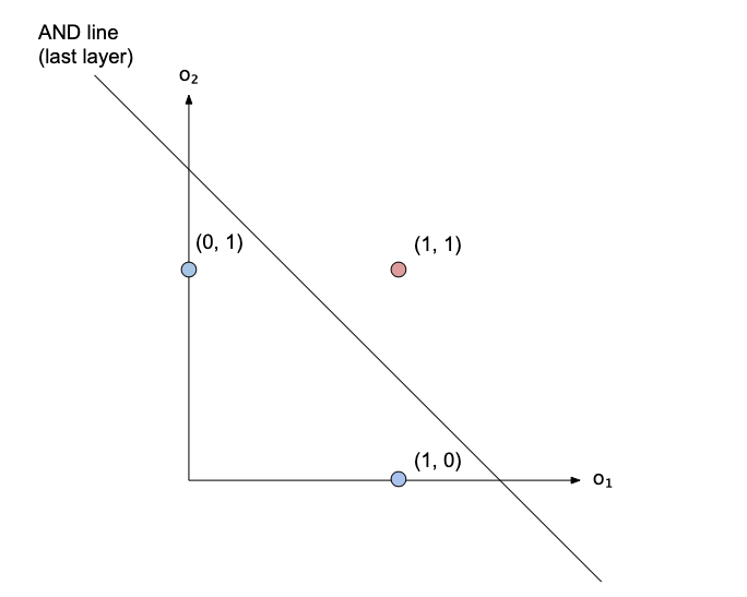
Two points have collapsed onto each other in (1, 1), and those are the points of the XOR! So it’s now possible to separate the XOR vs the other points with just a line. This is what the last layer will do: it will find a line that separates those three points! That line, in our case, corresponds to an AND.
Yet another perspective
Another way of looking at it is that each neuron is trying to find a relationship between its inputs so that further neurons can better use them.
So that, in our XOR network, the first neuron has found a useful relationship of the inputs (the OR relationship), the second neuron has found the NAND relationship, and the third neuron has found a relationship between those relationships (the AND relationship).
The more layers I add, the more relationships of relationships I will have, so things can get pretty abstract. That’s why people say the first layers “extract” simple features, while deeper layers combine those features to model more complex concepts.
Remember that those relationships are found by training the network (I have not explained how), which in turn means finding the w and b parameters for each neuron.
Other types of networks
In this post, I limited myself to a simple fully-connected feedforward network (a network in which all neurons of a layer are connected to the ones in the next layer and the connections are only forward).
There are many other types of networks, for example with different topologies, different activation functions, or even networks where the linear combinations in the neurons are replaced with something more complex.
One example is convolutional networks where convolution is applied instead of linear combinations.
This doesn’t change the modeling power of the network, as a simple fully-connected feedforward network can represent all the continuous function (as stated by the universal approximation theorem mentioned above).
But building a “structure” into the network (like a convolution) will make the training easier, since the training algorithm won’t have to figure out what a convolution is by itself. That could also be counter-productive, in cases where convolutions might not help that much (e.g. the principle of locality is not applicable), but that’s the topic for another post!
In the meantime, I hope I have given you a few different perspectives on how to look at neural networks.
1,072 total views, 2 views today